Medical Imaging

Helpers for working with DICOM files

Patching

---

source

get_dicom_files

 get_dicom_files (path, recurse=True, folders=None)

Get dicom files in path recursively, only in folders, if specified.

---

source

Path.dcmread

 Path.dcmread (fn:pathlib.Path, force=False)

Open a DICOM file

fastai.medical.imaging uses pydicom.dcmread to read a DICOM file. To view the header of a DICOM, specify the path of a test file and call dcmread.

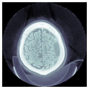
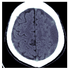
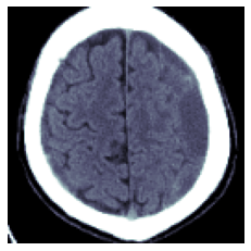
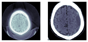
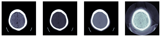
TEST_DCM = Path('images/sample.dcm')
dcm = TEST_DCM.dcmread()
dcm

Dataset.file_meta -------------------------------
(0002, 0000) File Meta Information Group Length  UL: 176
(0002, 0001) File Meta Information Version       OB: b'\x00\x01'
(0002, 0002) Media Storage SOP Class UID         UI: CT Image Storage
(0002, 0003) Media Storage SOP Instance UID      UI: 9999.180975792154576730321054399332994563536
(0002, 0010) Transfer Syntax UID                 UI: Explicit VR Little Endian
(0002, 0012) Implementation Class UID            UI: 1.2.40.0.13.1.1.1
(0002, 0013) Implementation Version Name         SH: 'dcm4che-1.4.38'
-------------------------------------------------
(0008, 0018) SOP Instance UID                    UI: ID_e0cc6a4b5
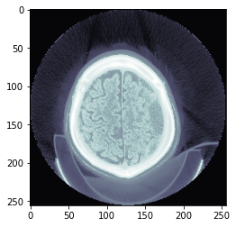
(0008, 0060) Modality                            CS: 'CT'
(0010, 0020) Patient ID                          LO: 'ID_a107dd7f'
(0020, 000d) Study Instance UID                  UI: ID_6468bdd34a
(0020, 000e) Series Instance UID                 UI: ID_4be303ae64
(0020, 0010) Study ID                            SH: ''
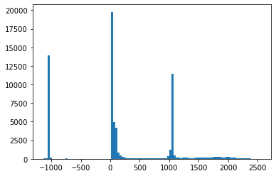
(0020, 0032) Image Position (Patient)            DS: [-125.000, -122.268, 115.936]
(0020, 0037) Image Orientation (Patient)         DS: [1.000000, 0.000000, 0.000000, 0.000000, 0.978148, -0.207912]
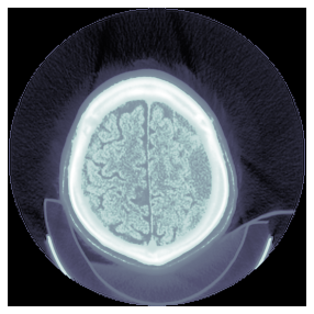
(0028, 0002) Samples per Pixel                   US: 1
(0028, 0004) Photometric Interpretation          CS: 'MONOCHROME2'
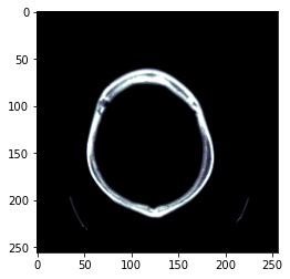
(0028, 0010) Rows                                US: 256
(0028, 0011) Columns                             US: 256
(0028, 0030) Pixel Spacing                       DS: [0.488281, 0.488281]
(0028, 0100) Bits Allocated                      US: 16
(0028, 0101) Bits Stored                         US: 16
(0028, 0102) High Bit                            US: 15
(0028, 0103) Pixel Representation                US: 1
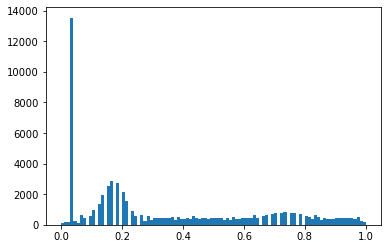
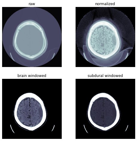
(0028, 1050) Window Center                       DS: "40.0"
(0028, 1051) Window Width                        DS: "100.0"
(0028, 1052) Rescale Intercept                   DS: "-1024.0"
(0028, 1053) Rescale Slope                       DS: "1.0"
(7fe0, 0010) Pixel Data                          OW: Array of 131072 elements

type(dcm)

pydicom.dataset.FileDataset

---

source

TensorDicom

 TensorDicom (x, **kwargs)

Inherits from TensorImage and converts the pixel_array into a TensorDicom

---

source

PILDicom

 PILDicom ()

Base class for a Pillow Image that can show itself and convert to a Tensor

---

source

Path.png16read

 Path.png16read ()

---

Dataset.pixels

 Dataset.pixels ()

pixel_array as a tensor

dcm.pixels

tensor([[-1024., -1024., -1024.,  ..., -1024., -1024., -1024.],
        [-1024., -1024., -1024.,  ..., -1024., -1024., -1024.],
        [-1024., -1024., -1024.,  ..., -1024., -1024., -1024.],
        ...,
        [-1024., -1024., -1024.,  ..., -1024., -1024., -1024.],
        [-1024., -1024., -1024.,  ..., -1024., -1024., -1024.],
        [-1024., -1024., -1024.,  ..., -1024., -1024., -1024.]])

---

Dataset.scaled_px

 Dataset.scaled_px ()

pixels scaled by RescaleSlope and RescaleIntercept

scaled_px uses RescaleSlope and RescaleIntercept values to correctly scale the image so that they represent the correct tissue densities. You can observe what scaled_px does by viewing the the pixel distribution of a dicom image. The histogram below displays the current pixel distribution which shows a pixel range between -1133 and 2545.

plt.hist(dcm.pixels.flatten().numpy());

As shown in the header of the test image the RescaleIntercept has a value of -1024.0 and a RescaleSlope value of 1.0. scaled_px will scale the pixels by these values.

plt.hist(dcm.scaled_px.flatten().numpy());

The pixel distibution is now between -2157 and 1521

---

source

array_freqhist_bins

 array_freqhist_bins (n_bins=100)

A numpy based function to split the range of pixel values into groups, such that each group has around the same number of pixels

---

source

Tensor.freqhist_bins

 Tensor.freqhist_bins (n_bins=100)

A function to split the range of pixel values into groups, such that each group has around the same number of pixels

For example with n_bins set to 1 this means the bins will be split into 3 distinct bins (the beginning, the end and the number of bins specified by n_bins.

t_bin = dcm.pixels.freqhist_bins(n_bins=1)
t_bin

tensor([-1076.,    40.,  2375.])

plt.hist(t_bin.numpy(), bins=t_bin, color='c')
plt.plot(t_bin, torch.linspace(0,1,len(t_bin)));

with n_bins at 100

t_bin = dcm.pixels.freqhist_bins(n_bins=100)
t_bin

tensor([-1076., -1026., -1024., -1021.,    28.,    30.,    31.,    32.,    33.,
           34.,    35.,    36.,    37.,    38.,    39.,    40.,    41.,    42.,
           44.,    48.,    52.,    58.,    66.,    72.,    76.,    80.,    85.,
           91.,    94.,    98.,   103.,   111.,   123.,   161.,   219.,   478.,
          829.,   999.,  1027.,  1038.,  1044.,  1047.,  1049.,  1050.,  1051.,
         1052.,  1053.,  1054.,  1055.,  1056.,  1057.,  1058.,  1059.,  1060.,
         1062.,  1066.,  1108.,  1265.,  1453.,  1616.,  1741.,  1838.,  1943.,
         2051.,  2220.,  2375.])

plt.hist(t_bin.numpy(), bins=t_bin, color='c'); plt.plot(t_bin, torch.linspace(0,1,len(t_bin)));

---

source

Tensor.hist_scaled_pt

 Tensor.hist_scaled_pt (brks=None)

---

source

Tensor.hist_scaled

 Tensor.hist_scaled (brks=None)

Scales a tensor using freqhist_bins to values between 0 and 1

The test image has pixel values that range between -1000 and 2500

plt.hist(dcm.pixels.flatten().numpy(), bins=100);

hist_scaled provides a way of scaling the input pixel values to between 0 and 1

tensor_hists = dcm.pixels.hist_scaled()
plt.hist(tensor_hists.flatten().numpy(), bins=100);

---

Dataset.hist_scaled

 Dataset.hist_scaled (brks=None, min_px=None, max_px=None)

Pixels scaled to a min_px and max_px value

data_scaled = dcm.hist_scaled()
plt.imshow(data_scaled, cmap=plt.cm.bone);

data_scaled = dcm.hist_scaled(min_px=100, max_px=1000)
plt.imshow(data_scaled, cmap=plt.cm.bone);

Dicom images can contain a high amount of voxel values and windowing can be thought of as a means of manipulating these values in order to change the apperance of the image so particular structures are highlighted. A window has 2 values:

• l = window level or center aka brightness
• w = window width or range aka contrast

---

source

Tensor.windowed

 Tensor.windowed (w, l)

Scale pixel intensity by window width and window level

---

Dataset.windowed

 Dataset.windowed (w, l)

plt.imshow(dcm.windowed(*dicom_windows.brain), cmap=plt.cm.bone);

---

source

TensorCTScan

 TensorCTScan (x, **kwargs)

Inherits from TensorImageBW and converts the pixel_array into a TensorCTScan

tensor_ct = TensorCTScan(dcm.pixel_array)
tensor_ct.show();

---

source

PILCTScan

 PILCTScan ()

Base class for a Pillow Image that can show itself and convert to a Tensor

---

Dataset.show

 Dataset.show (scale=True, cmap=<matplotlib.colors.LinearSegmentedColormap
               object at 0x7f3cfade6680>, min_px=-1100, max_px=None,
               ax=None, figsize=None, title=None, ctx=None, norm=None,
               aspect=None, interpolation=None, alpha=None, vmin=None,
               vmax=None, origin=None, extent=None,
               interpolation_stage=None, filternorm=True, filterrad=4.0,
               resample=None, url=None, data=None)

Display a normalized dicom image by default

scales = False, True, dicom_windows.brain, dicom_windows.subdural
titles = 'raw','normalized','brain windowed','subdural windowed'
for s,a,t in zip(scales, subplots(2,2,imsize=4)[1].flat, titles):
    dcm.show(scale=s, ax=a, title=t)

dcm.show(cmap=plt.cm.gist_ncar, figsize=(6,6))

Some dicom datasets such as the The Thyroid Segmentation in Ultrasonography Dataset is a dataset where each image has multiple frames per file (hundreds in this case). By default the show function will display 1 frame but if the dataset has multiple frames you can specify the number of frames to view.

---

Dataset.show

 Dataset.show (frames=1, scale=True,
               cmap=<matplotlib.colors.LinearSegmentedColormap object at
               0x7f3cfade6680>, min_px=-1100, max_px=None, **kwargs)

Adds functionality to view dicom images where each file may have more than 1 frame

dcm.show()

---

Dataset.pct_in_window

 Dataset.pct_in_window (dcm:pydicom.dataset.Dataset, w, l)

% of pixels in the window (w,l)

dcm.pct_in_window(*dicom_windows.brain)

0.19049072265625

pct_in_window can be used to check what percentage of the image is composed of meaningful pixels (pixels within the specified window)

---

source

uniform_blur2d

 uniform_blur2d (x, s)

Uniformly apply blurring

ims = dcm.hist_scaled(), uniform_blur2d(dcm.hist_scaled(), 20), uniform_blur2d(dcm.hist_scaled(), 50)
show_images(ims, titles=('original', 'blurred 20', 'blurred 50'))

---

source

gauss_blur2d

 gauss_blur2d (x, s)

Apply gaussian_blur2d kornia filter

ims = dcm.hist_scaled(), gauss_blur2d(dcm.hist_scaled(), 20), gauss_blur2d(dcm.hist_scaled(), 50)
show_images(ims, titles=('original', 'gauss_blur 20', 'gauss_blur 50'))

Images are often affected by random variations in intensity values, called noise. Gaussian noise contains variatons in intensity that are drawn from a Gaussian or normal distribution. A Guassian filter is usually used to blur edges and remove smaller or thinner areas in order to preserve the most important information

---

source

Tensor.mask_from_blur

 Tensor.mask_from_blur (x:torch.Tensor, window, sigma=0.3, thresh=0.05,
                        remove_max=True)

Create a mask from the blurred image

---

Dataset.mask_from_blur

 Dataset.mask_from_blur (x:pydicom.dataset.Dataset, window, sigma=0.3,
                         thresh=0.05, remove_max=True)

Create a mask from the blurred image

mask = dcm.mask_from_blur(dicom_windows.brain, sigma=0.9, thresh=0.1, remove_max=True)
wind = dcm.windowed(*dicom_windows.brain)

_,ax = subplots(1,3)
show_image(wind, ax=ax[0], title='window')
show_image(mask, alpha=0.5, cmap=plt.cm.Reds, ax=ax[1], title='mask')
show_image(wind, ax=ax[2])
show_image(mask, alpha=0.5, cmap=plt.cm.Reds, ax=ax[2], title='window and mask');

---

source

mask2bbox

 mask2bbox (mask)

bbs = mask2bbox(mask)
lo,hi = bbs
show_image(wind[lo[0]:hi[0],lo[1]:hi[1]]);

---

source

crop_resize

 crop_resize (x, crops, new_sz)

px256 = crop_resize(to_device(wind[None]), bbs[...,None], 128)[0]
show_image(px256)
px256.shape

torch.Size([1, 128, 128])

Comparing the original image with the image from using the mask and crop_resize function

_,axs = subplots(1,2)
dcm.show(ax=axs[0])
show_image(px256, ax=axs[1]);

---

source

Tensor.to_nchan

 Tensor.to_nchan (x:torch.Tensor, wins, bins=None)

---

Dataset.to_nchan

 Dataset.to_nchan (x:pydicom.dataset.Dataset, wins, bins=None)

to_nchan takes a tensor or a dicom as the input and returns multiple one channel images (the first depending on the choosen windows and a normalized image). Setting bins to 0 only returns the windowed image.

show_images(dcm.to_nchan([dicom_windows.brain], bins=0))

show_images(dcm.to_nchan([dicom_windows.brain], bins=None))

---

source

Tensor.to_3chan

 Tensor.to_3chan (x:torch.Tensor, win1, win2, bins=None)

---

Dataset.to_3chan

 Dataset.to_3chan (x:pydicom.dataset.Dataset, win1, win2, bins=None)

show_images(dcm.to_nchan([dicom_windows.brain,dicom_windows.subdural,dicom_windows.abdomen_soft]))

---

save_jpg’]

*Built-in mutable sequence.

If no argument is given, the constructor creates a new empty list. The argument must be an iterable if specified.*

---

to_uint16’]

*Built-in mutable sequence.

If no argument is given, the constructor creates a new empty list. The argument must be an iterable if specified.*

---

save_tif16’]

*Built-in mutable sequence.

If no argument is given, the constructor creates a new empty list. The argument must be an iterable if specified.*

_,axs=subplots(1,2)
with tempfile.TemporaryDirectory() as f:
    f = Path(f)
    dcm.save_jpg(f/'test.jpg', [dicom_windows.brain,dicom_windows.subdural])
    show_image(Image.open(f/'test.jpg'), ax=axs[0])
    dcm.save_tif16(f/'test.tif')
    show_image(Image.open(str(f/'test.tif')), ax=axs[1]);

---

Dataset.set_pixels

 Dataset.set_pixels (px)

---

Dataset.zoom

 Dataset.zoom (ratio)

Zoom image by specified ratio

Check to see the current size of the dicom image

dcm.pixel_array.shape

(256, 256)

dcm.zoom(7.0)
dcm.show(); dcm.pixel_array.shape

---

Dataset.zoom_to

 Dataset.zoom_to (sz)

Change image size to specified pixel size

dcm.zoom_to(200); dcm.pixel_array.shape

(200, 200)

---

Dataset.shape

 Dataset.shape ()

Returns the shape of a dicom image as rows and columns

dcm2 = TEST_DCM.dcmread()
dcm2.zoom_to(90)
test_eq(dcm2.shape, (90,90))

dcm2 = TEST_DCM.dcmread()
dcm2.zoom(0.25)
dcm2.show()

---

Dataset.as_dict

 Dataset.as_dict (px_summ=True, window=(80, 40))

Convert the header of a dicom into a dictionary

as_dict takes in 2 parameters: px_summ which by default is set to True and this returns additional stats such as minimal pixel value, maximum pixel value, the mean pixel value and the image standard deviation. The window parameter calculates the pct_in_window value depending on the window that is specified.

dcm.as_dict(px_summ=True, window=dicom_windows.brain);

Creating a dataframe of the values within the header of the dicom

pneumothorax_source = untar_data(URLs.SIIM_SMALL)
items = get_dicom_files(pneumothorax_source, recurse=True,  folders='train')
dicom_dataframe = pd.DataFrame.from_dicoms(items, window=dicom_windows.brain, px_summ=True)
dicom_dataframe.head(2).T.tail(5)

	0	1
img_min	0	0
img_max	254	250
img_mean	160.398	114.525
img_std	53.8549	70.7523
img_pct_window	0.0870295	0.326269

---

source

DicomSegmentationDataLoaders

 DicomSegmentationDataLoaders (*loaders, path:str|pathlib.Path='.',
                               device=None)

Basic wrapper around DICOM DataLoaders with factory methods for segmentation problems

path = untar_data(URLs.TCGA_SMALL)
codes = np.loadtxt(path/'codes.txt', dtype=str)
fnames = get_dicom_files(path/'dicoms')
label_func = lambda o: path/'labels'/f'{o.stem}.png'

dls = DicomSegmentationDataLoaders.from_label_func(path, fnames, label_func, codes=codes, bs=4)
dls.show_batch()