from fastai.test_utils import *Hyperparam schedule
Callback and helper functions to schedule any hyper-parameter
Annealing
annealer
def annealer(
    f
):
Decorator to make f return itself partially applied.
This is the decorator we will use for all of our scheduling functions, as it transforms a function taking (start, end, pos) to something taking (start, end) and return a function depending of pos.
sched_exp
def sched_exp(
    start, end, pos
):
Call self as a function.
sched_no
def sched_no(
    start, end, pos
):
Call self as a function.
sched_cos
def sched_cos(
    start, end, pos
):
Call self as a function.
sched_lin
def sched_lin(
    start, end, pos
):
Call self as a function.
annealings = "NO LINEAR COS EXP".split()
p = torch.linspace(0.,1,100)
fns = [SchedNo, SchedLin, SchedCos, SchedExp]
for fn, t in zip(fns, annealings):
plt.plot(p, [fn(2, 1e-2)(o) for o in p], label=t)
f = SchedPoly(2,1e-2,0.5)
plt.plot(p, [f(o) for o in p], label="POLY(0.5)")
plt.legend();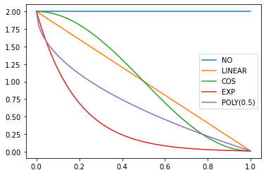
SchedLin
def SchedLin(
    start, end
):
Linear schedule function from start to end
sched = SchedLin(0, 2)
test_eq(L(map(sched, [0., 0.25, 0.5, 0.75, 1.])), [0., 0.5, 1., 1.5, 2.])SchedCos
def SchedCos(
    start, end
):
Cosine schedule function from start to end
sched = SchedCos(0, 2)
test_close(L(map(sched, [0., 0.25, 0.5, 0.75, 1.])), [0., 0.29289, 1., 1.70711, 2.])SchedNo
def SchedNo(
    start, end
):
Constant schedule function with start value
sched = SchedNo(0, 2)
test_close(L(map(sched, [0., 0.25, 0.5, 0.75, 1.])), [0., 0., 0., 0., 0.])SchedExp
def SchedExp(
    start, end
):
Exponential schedule function from start to end
sched = SchedExp(1, 2)
test_close(L(map(sched, [0., 0.25, 0.5, 0.75, 1.])), [1., 1.18921, 1.41421, 1.68179, 2.])SchedPoly
def SchedPoly(
    start, end, power
):
Polynomial schedule (of power) function from start to end
sched = SchedPoly(0, 2, 2)
test_close(L(map(sched, [0., 0.25, 0.5, 0.75, 1.])), [0., 0.125, 0.5, 1.125, 2.])
p = torch.linspace(0.,1,100)
pows = [0.5,1.,2.]
for e in pows:
f = SchedPoly(2, 0, e)
plt.plot(p, [f(o) for o in p], label=f'power {e}')
plt.legend();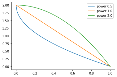
combine_scheds
def combine_scheds(
    pcts, scheds
):
Combine scheds according to pcts in one function
pcts must be a list of positive numbers that add up to 1 and is the same length as scheds. The generated function will use scheds[0] from 0 to pcts[0] then scheds[1] from pcts[0] to pcts[0]+pcts[1] and so forth.
p = torch.linspace(0.,1,100)
f = combine_scheds([0.3,0.7], [SchedCos(0.3,0.6), SchedCos(0.6,0.2)])
plt.plot(p, [f(o) for o in p]);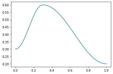
p = torch.linspace(0.,1,100)
f = combine_scheds([0.3,0.2,0.5], [SchedLin(0.,1.), SchedNo(1.,1.), SchedCos(1., 0.)])
plt.plot(p, [f(o) for o in p]);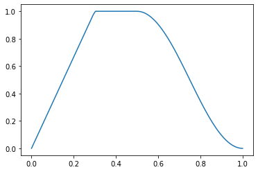
combined_cos
def combined_cos(
    pct, start, middle, end
):
Return a scheduler with cosine annealing from start→middle & middle→end
This is a useful helper function for the 1cycle policy. pct is used for the start to middle part, 1-pct for the middle to end. Handles floats or collection of floats. For example:
f = combined_cos(0.25,0.5,1.,0.)
plt.plot(p, [f(o) for o in p]);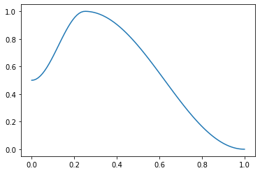
ParamScheduler
def ParamScheduler(
    scheds
):
Schedule hyper-parameters according to scheds
scheds is a dictionary with one key for each hyper-parameter you want to schedule, with either a scheduler or a list of schedulers as values (in the second case, the list must have the same length as the the number of parameters groups of the optimizer).
learn = synth_learner()
sched = {'lr': SchedLin(1e-3, 1e-2)}
learn.fit(1, cbs=ParamScheduler(sched))
n = len(learn.dls.train)
test_close(learn.recorder.hps['lr'], [1e-3 + (1e-2-1e-3) * i/n for i in range(n)])| epoch | train_loss | valid_loss | time |
|---|---|---|---|
| 0 | 11.929138 | 4.039281 | 00:00 |
ParamScheduler.before_fit
def before_fit():Initialize container for hyper-parameters
ParamScheduler.before_batch
def before_batch():Set the proper hyper-parameters in the optimizer
ParamScheduler.after_batch
def after_batch():Record hyper-parameters of this batch
ParamScheduler.after_fit
def after_fit():Save the hyper-parameters in the recorder if there is one
Learner.fit_one_cycle
def fit_one_cycle(
    n_epoch, lr_max:NoneType=None, div:float=25.0, div_final:float=100000.0, pct_start:float=0.25, wd:NoneType=None,
    moms:NoneType=None, cbs:NoneType=None, reset_opt:bool=False, start_epoch:int=0
):
Fit self.model for n_epoch using the 1cycle policy.
The 1cycle policy was introduced by Leslie N. Smith et al. in Super-Convergence: Very Fast Training of Neural Networks Using Large Learning Rates. It schedules the learning rate with a cosine annealing from lr_max/div to lr_max then lr_max/div_final (pass an array to lr_max if you want to use differential learning rates) and the momentum with cosine annealing according to the values in moms. The first phase takes pct_start of the training. You can optionally pass additional cbs and reset_opt.
#Integration test: training a few epochs should make the model better
learn = synth_learner(lr=1e-2)
xb,yb = learn.dls.one_batch()
init_loss = learn.loss_func(learn.model(xb), yb)
learn.fit_one_cycle(2)
xb,yb = learn.dls.one_batch()
final_loss = learn.loss_func(learn.model(xb), yb)
assert final_loss < init_loss| epoch | train_loss | valid_loss | time |
|---|---|---|---|
| 0 | 19.444899 | 6.755066 | 00:00 |
| 1 | 9.919473 | 1.044571 | 00:00 |
#Scheduler test
lrs,moms = learn.recorder.hps['lr'],learn.recorder.hps['mom']
test_close(lrs,  [combined_cos(0.25,1e-2/25,1e-2,1e-7)(i/20) for i in range(20)])
test_close(moms, [combined_cos(0.25,0.95,0.85,0.95)(i/20) for i in range(20)])Recorder.plot_sched
def plot_sched(
    keys:NoneType=None, figsize:NoneType=None
):
Call self as a function.
learn = synth_learner()
learn.fit_one_cycle(2)| epoch | train_loss | valid_loss | time |
|---|---|---|---|
| 0 | 5.406837 | 5.305011 | 00:00 |
| 1 | 5.058437 | 4.899223 | 00:00 |
learn.recorder.plot_sched()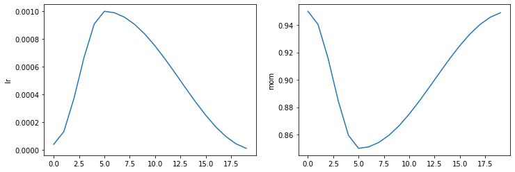
Learner.fit_flat_cos
def fit_flat_cos(
    n_epoch, lr:NoneType=None, div_final:float=100000.0, pct_start:float=0.75, wd:NoneType=None, cbs:NoneType=None,
    reset_opt:bool=False, start_epoch:int=0
):
Fit self.model for n_epoch at flat lr before a cosine annealing.
learn = synth_learner()
learn.fit_flat_cos(2)| epoch | train_loss | valid_loss | time |
|---|---|---|---|
| 0 | 10.588930 | 7.106113 | 00:00 |
| 1 | 8.943380 | 5.016665 | 00:00 |
learn.recorder.plot_sched()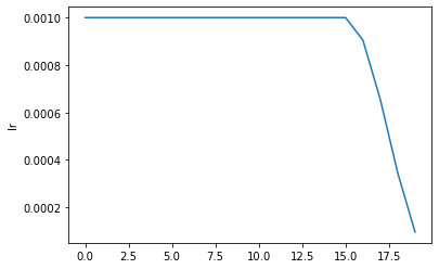
Learner.fit_sgdr
def fit_sgdr(
    n_cycles, cycle_len, lr_max:NoneType=None, cycle_mult:int=2, cbs:NoneType=None, reset_opt:bool=False,
    wd:NoneType=None, start_epoch:int=0
):
Fit self.model for n_cycles of cycle_len using SGDR.
This schedule was introduced by Ilya Loshchilov et al. in SGDR: Stochastic Gradient Descent with Warm Restarts. It consists of n_cycles that are cosine annealings from lr_max (defaults to the Learner lr) to 0, with a length of cycle_len * cycle_mult**i for the i-th cycle (first one is cycle_len-long, then we multiply the length by cycle_mult at each epoch). You can optionally pass additional cbs and reset_opt.
learn = synth_learner()
with learn.no_logging(): learn.fit_sgdr(3, 1)
test_eq(learn.n_epoch, 7)
iters = [k * len(learn.dls.train) for k in [0,1,3,7]]
for i in range(3):
    n = iters[i+1]-iters[i]
    #The start of a cycle can be mixed with the 0 of the previous cycle with rounding errors, so we test at +1
    test_close(learn.recorder.lrs[iters[i]+1:iters[i+1]], [SchedCos(learn.lr, 0)(k/n) for k in range(1,n)])

learn.recorder.plot_sched()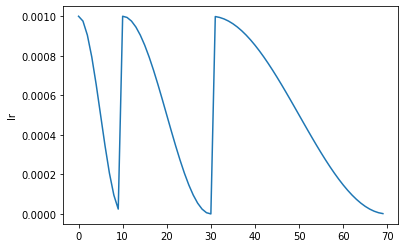
Learner.fine_tune
def fine_tune(
    epochs, base_lr:float=0.002, freeze_epochs:int=1, lr_mult:int=100, pct_start:float=0.3, div:float=5.0,
    lr_max:NoneType=None, div_final:float=100000.0, wd:NoneType=None, moms:NoneType=None, cbs:NoneType=None,
    reset_opt:bool=False, start_epoch:int=0
):
Fine tune with Learner.freeze for freeze_epochs, then with Learner.unfreeze for epochs, using discriminative LR.
learn.fine_tune(1)| epoch | train_loss | valid_loss | time |
|---|---|---|---|
| 0 | 2.428970 | 1.740237 | 00:00 |
| epoch | train_loss | valid_loss | time |
|---|---|---|---|
| 0 | 2.019952 | 1.616970 | 00:00 |
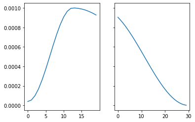
Resume training from checkpoint
To enable resuming from checkpoint make sure to save model and optimizer state. This can be done using SaveModelCallback setting (with_opt=True). If training is interrupted define learn using the same parameters as before, load model from checkpoint and pass start_epoch to fit call. The training will be resumed from start_epoch with properly scheduled lr.
with tempfile.TemporaryDirectory() as d:
    learn1 = synth_learner(path=d, cbs=SaveModelCallback(with_opt=True, fname="ckpt"))
    learn1.fit_one_cycle(5, cbs=InterruptCallback(2))

    learn2 = synth_learner(path=d)
    learn2 = learn2.load("ckpt")
    learn2.fit_one_cycle(5, start_epoch=2)

    fig, axs = plt.subplots(1,2, sharey=True)
    axs[0].plot(learn1.recorder.lrs)
axs[1].plot(learn2.recorder.lrs)| epoch | train_loss | valid_loss | time |
|---|---|---|---|
| 0 | 18.930223 | 14.100439 | 00:00 |
| 1 | 17.092665 | 10.603369 | 00:00 |
Better model found at epoch 0 with valid_loss value: 14.100439071655273.
Better model found at epoch 1 with valid_loss value: 10.603368759155273.| epoch | train_loss | valid_loss | time |
|---|---|---|---|
| 0 | 00:00 | ||
| 1 | 00:00 | ||
| 2 | 11.456764 | 10.057186 | 00:00 |
| 3 | 10.287196 | 8.694046 | 00:00 |
| 4 | 9.585465 | 8.422710 | 00:00 |
LRFinder
def LRFinder(
    start_lr:float=1e-07, end_lr:int=10, num_it:int=100, stop_div:bool=True
):
Training with exponentially growing learning rate
from fastai.vision.all import *set_seed(99, True)
path = untar_data(URLs.PETS)/'images'
image_files = get_image_files(path)
if sys.platform == "win32" and IN_NOTEBOOK:
image_files = random.choices(image_files, k=int(len(image_files)/8))
print("Randomly select 1/8 files in NOTEBOOK on Windows to save time")
# pickle can't serializer lamda function.
def _label_func(x):
return x[0].isupper()
dls = ImageDataLoaders.from_name_func(
path, image_files, valid_pct=0.2,
label_func=_label_func, item_tfms=Resize(224))
learn = vision_learner(dls, resnet18)
learn.fit(1)
learn.opt.state_dict()['state'][1]['grad_avg']| epoch | train_loss | valid_loss | time |
|---|---|---|---|
| 0 | 0.086690 | 0.016682 | 00:33 |
tensor([-5.8191e-04, -2.2443e-03,  0.0000e+00, -1.2517e-03,  0.0000e+00,
        -1.4744e-03, -3.6433e-04,  0.0000e+00,  9.3745e-03,  0.0000e+00,
         5.1993e-03, -1.5093e-02, -4.0410e-03,  0.0000e+00,  7.1963e-03,
        -6.6033e-03, -3.3354e-03, -2.9191e-03, -1.5054e-03, -1.3179e-03,
         8.7333e-03, -1.1155e-02, -9.6656e-04,  1.6653e-02,  9.5839e-04,
         8.4995e-03, -2.8187e-02,  3.1579e-03, -9.3051e-04, -2.3887e-03,
        -7.3557e-04, -1.4501e-02, -6.2110e-03,  1.9949e-03, -7.0233e-03,
         1.2792e-02,  0.0000e+00,  1.0687e-03,  0.0000e+00, -4.2413e-04,
         2.9628e-03,  7.2686e-03, -9.7241e-03, -4.9941e-04,  1.7408e-02,
        -9.2441e-03, -9.7731e-03, -9.9393e-03,  0.0000e+00, -2.1448e-03,
         2.7660e-03, -3.1110e-03,  5.9454e-05, -1.4412e-03, -6.1454e-04,
        -1.6537e-03,  1.7001e-02,  1.4041e-02, -6.2878e-03,  2.0800e-02,
        -1.2900e-02, -1.2626e-02, -2.6591e-03,  3.9685e-03], device='cuda:0')
with tempfile.TemporaryDirectory() as d:
learn = synth_learner(path=Path(d))
init_a,init_b = learn.model.a,learn.model.b
with learn.no_logging(): learn.fit(20, cbs=LRFinder(num_it=100))
assert len(learn.recorder.lrs) <= 100
test_eq(len(learn.recorder.lrs), len(learn.recorder.losses))
#Check stop if diverge
if len(learn.recorder.lrs) < 100: assert learn.recorder.losses[-1] > 4 * min(learn.recorder.losses)
#Test schedule
test_eq(learn.recorder.lrs, [SchedExp(1e-7, 10)(i/100) for i in range_of(learn.recorder.lrs)])
#No validation data
test_eq([len(v) for v in learn.recorder.values], [1 for _ in range_of(learn.recorder.values)])
#Model loaded back properly
test_eq(learn.model.a, init_a)
test_eq(learn.model.b, init_b)
test_eq(learn.opt.state_dict()['state'], [{}, {}])LRFinder.before_fit
def before_fit():Initialize container for hyper-parameters and save the model
LRFinder.before_batch
def before_batch():Set the proper hyper-parameters in the optimizer
LRFinder.after_batch
def after_batch():Record hyper-parameters of this batch and potentially stop training
LRFinder.before_validate
def before_validate():Skip the validation part of training
Suggestion Methods
There are a few methodologies for suggesting a learning rate automatically and these as we will see can further be passed into lr_find. Currently four methods are supported, however to write your own it should look like a function that can accept LRFinder’s returned lrs, losses, as well as the num_it. Your function should return an x,y coordinate that can be plotted, such as below:
def myfunc(lrs:list, losses:list, num_it:int) -> tuple(float, tuple(float,int)):
    ...
    return suggestion, (suggestion,loss_idx)
If there are any more parameters to be passed in, you should pass in your func as a partial and specify them yourself, such as:
def myfunc(lrs:list, losses:list, num_it:int, pct_reduction:float) -> tuple(float, tuple(float,int)):
    ...
    return suggestion, (suggestion,loss_idx)
f = partial(myfunc, pct_reduction=.2)valley
def valley(
    lrs:list, losses:list, num_it:int
):
Suggests a learning rate from the longest valley and returns its index
The valley algorithm was developed by ESRI and takes the steepest slope roughly 2/3 through the longest valley in the LR plot, and is also the default for Learner.lr_find
slide
def slide(
    lrs:list, losses:list, num_it:int, lr_diff:int=15, thresh:float=0.005, adjust_value:float=1.0
):
Suggests a learning rate following an interval slide rule and returns its index
The slide rule is an algorithm developed by Andrew Chang out of Novetta, and is detailed here.
minimum
def minimum(
    lrs:list, losses:list, num_it:int
):
Suggests a learning rate one-tenth the minumum before divergance and returns its index
steep
def steep(
    lrs:list, losses:list, num_it:int
)->(<class 'float'>, <class 'tuple'>):
Suggests a learning rate when the slope is the steepest and returns its index
Recorder.plot_lr_find
def plot_lr_find(
    skip_end:int=5, return_fig:bool=True, suggestions:NoneType=None, nms:NoneType=None, **kwargs
):
Plot the result of an LR Finder test (won’t work if you didn’t do learn.lr_find() before)
Learner.lr_find
def lr_find(
    start_lr:float=1e-07, end_lr:int=10, num_it:int=100, stop_div:bool=True, show_plot:bool=True,
    suggest_funcs:function=valley
):
Launch a mock training to find a good learning rate and return suggestions based on suggest_funcs as a named tuple
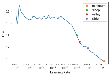
First introduced by Leslie N. Smith in Cyclical Learning Rates for Training Neural Networks, the LR Finder trains the model with exponentially growing learning rates from start_lr to end_lr for num_it and stops in case of divergence (unless stop_div=False) then plots the losses vs the learning rates with a log scale.
A variety of learning rate suggestion algorithms can be passed into the function, by default we use the valley paradigm.
with tempfile.TemporaryDirectory() as d:
    learn = synth_learner(path=Path(d))
    weights_pre_lr_find = L(learn.model.parameters())
    lr_min, lr_steep, lr_valley, lr_slide = learn.lr_find(suggest_funcs=(minimum, steep, valley, slide))
    weights_post_lr_find = L(learn.model.parameters())
test_eq(weights_pre_lr_find, weights_post_lr_find)
print(f"Minimum/10:\t{lr_min:.2e}\nSteepest point:\t{lr_steep:.2e}\nLongest valley:\t{lr_valley:.2e}\nSlide interval:\t{lr_slide:.2e}")
Minimum/10: 1.58e-01
Steepest point: 9.12e-03
Longest valley: 1.58e-02
Slide interval: 8.32e-02