model = nn.Sequential(nn.Linear(10,30), nn.BatchNorm1d(30), nn.Linear(30,2)).cuda()
model = convert_network(model, torch.float16)
for i,t in enumerate([torch.float16, torch.float32, torch.float16]):
test_eq(model[i].weight.dtype, t)
test_eq(model[i].bias.dtype, t)
model = nn.Sequential(nn.Linear(10,30), BatchNorm(30, ndim=1), nn.Linear(30,2)).cuda()
model = convert_network(model, torch.float16)
for i,t in enumerate([torch.float16, torch.float32, torch.float16]):
test_eq(model[i].weight.dtype, t)
test_eq(model[i].bias.dtype, t)Mixed precision training
A little bit of theory
A very nice and clear introduction to mixed precision training is this video from NVIDIA.
What’s half precision?
In neural nets, all the computations are usually done in single precision, which means all the floats in all the arrays that represent inputs, activations, weights… are 32-bit floats (FP32 in the rest of this post). An idea to reduce memory usage (and avoid those annoying cuda errors) has been to try and do the same thing in half-precision, which means using 16-bits floats (or FP16 in the rest of this post). By definition, they take half the space in RAM, and in theory could allow you to double the size of your model and double your batch size.
Another very nice feature is that NVIDIA developed its latest GPUs (the Volta generation) to take fully advantage of half-precision tensors. Basically, if you give half-precision tensors to those, they’ll stack them so that each core can do more operations at the same time, and theoretically gives an 8x speed-up (sadly, just in theory).
So training at half precision is better for your memory usage, way faster if you have a Volta GPU (still a tiny bit faster if you don’t since the computations are easiest). How do we do it? Super easily in pytorch, we just have to put .half() everywhere: on the inputs of our model and all the parameters. Problem is that you usually won’t see the same accuracy in the end (so it happens sometimes) because half-precision is… well… not as precise ;).
Problems with half-precision:
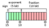
To understand the problems with half precision, let’s look briefly at what an FP16 looks like (more information here).

The sign bit gives us +1 or -1, then we have 5 bits to code an exponent between -14 and 15, while the fraction part has the remaining 10 bits. Compared to FP32, we have a smaller range of possible values (2e-14 to 2e15 roughly, compared to 2e-126 to 2e127 for FP32) but also a smaller offset.
For instance, between 1 and 2, the FP16 format only represents the number 1, 1+2e-10, 1+2*2e-10… which means that 1 + 0.0001 = 1 in half precision. That’s what will cause a certain numbers of problems, specifically three that can occur and mess up your training.
The weight update is imprecise: inside your optimizer, you basically do w = w - lr * w.grad for each weight of your network. The problem in performing this operation in half precision is that very often, w.grad is several orders of magnitude below w, and the learning rate is also small. The situation where w=1 and lr*w.grad is 0.0001 (or lower) is therefore very common, but the update doesn’t do anything in those cases.
Your gradients can underflow. In FP16, your gradients can easily be replaced by 0 because they are too low.
Your activations or loss can overflow. The opposite problem from the gradients: it’s easier to hit nan (or infinity) in FP16 precision, and your training might more easily diverge.
The solution: mixed precision training
To address those three problems, we don’t fully train in FP16 precision. As the name mixed training implies, some of the operations will be done in FP16, others in FP32. This is mainly to take care of the first problem listed above. For the next two there are additional tricks.
The main idea is that we want to do the forward pass and the gradient computation in half precision (to go fast) but the update in single precision (to be more precise). It’s okay if w and grad are both half floats, but when we do the operation w = w - lr * grad, we need to compute it in FP32. That way our 1 + 0.0001 is going to be 1.0001.
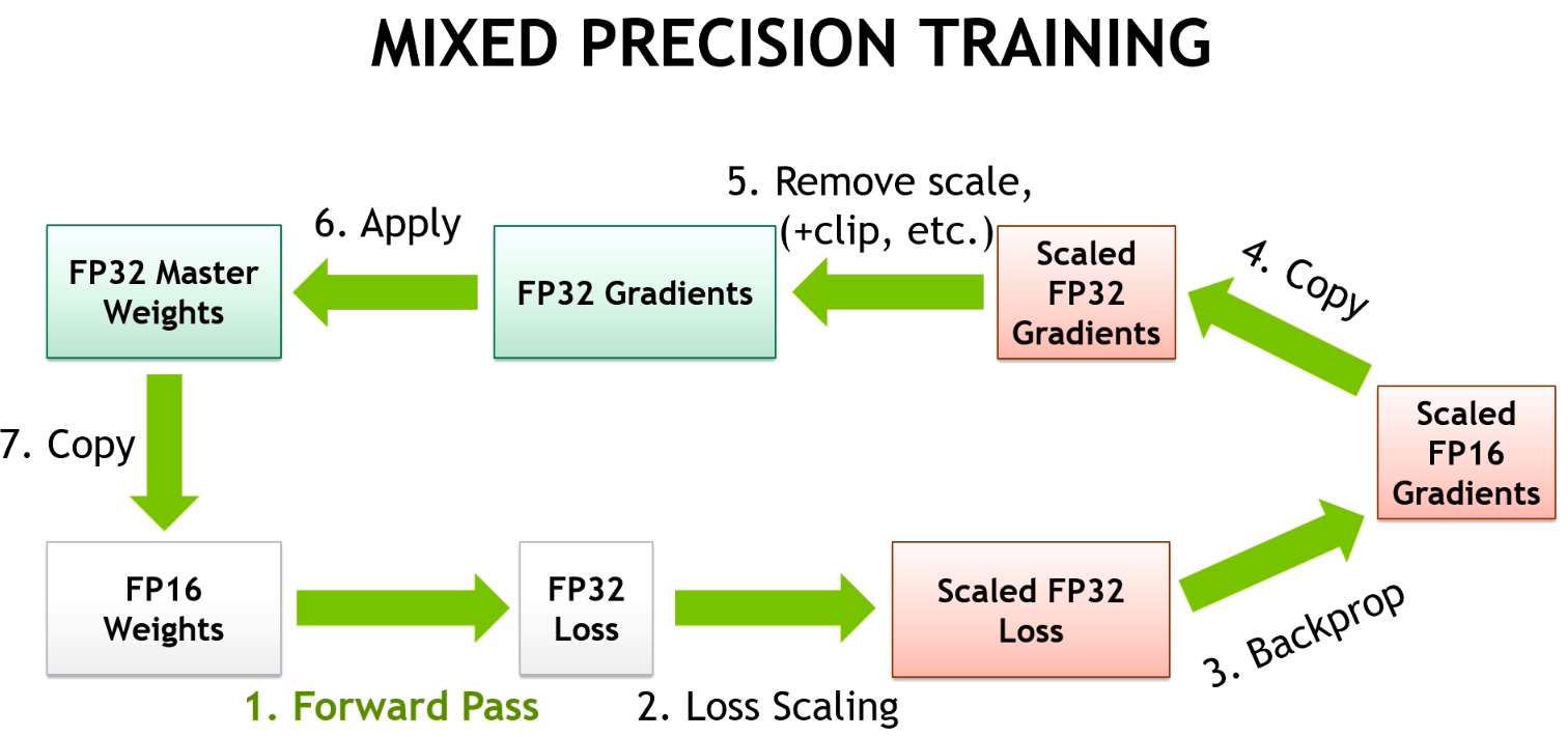
This is why we keep a copy of the weights in FP32 (called master model). Then, our training loop will look like:
- compute the output with the FP16 model, then the loss
- back-propagate the gradients in half-precision.
- copy the gradients in FP32 precision
- do the update on the master model (in FP32 precision)
- copy the master model in the FP16 model.
Note that we lose precision during step 5, and that the 1.0001 in one of the weights will go back to 1. But if the next update corresponds to add 0.0001 again, since the optimizer step is done on the master model, the 1.0001 will become 1.0002 and if we eventually go like this up to 1.0005, the FP16 model will be able to tell the difference.
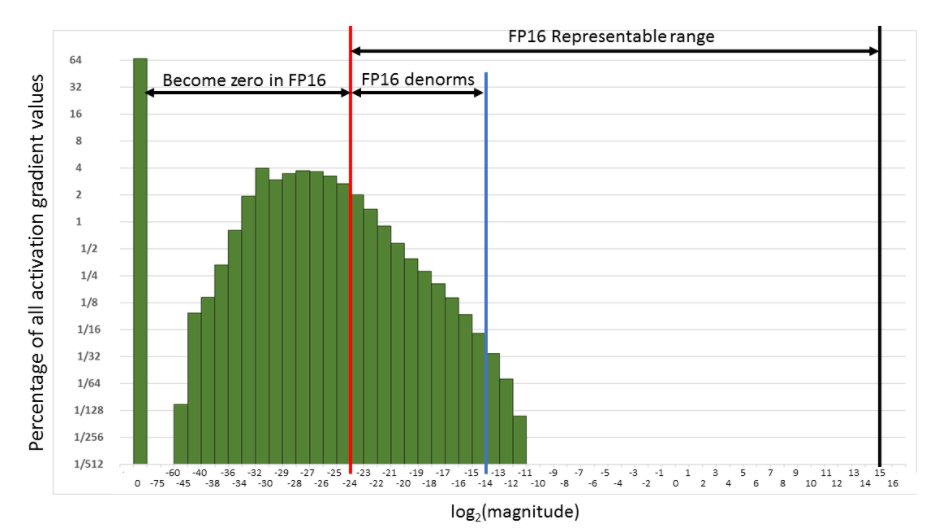
That takes care of problem 1. For the second problem, we use something called gradient scaling: to avoid the gradients getting zeroed by the FP16 precision, we multiply the loss by a scale factor (scale=512 for instance). That way we can push the gradients to the right in the next figure, and have them not become zero.

Of course we don’t want those 512-scaled gradients to be in the weight update, so after converting them into FP32, we can divide them by this scale factor (once they have no risks of becoming 0). This changes the loop to:
- compute the output with the FP16 model, then the loss.
- multiply the loss by scale then back-propagate the gradients in half-precision.
- copy the gradients in FP32 precision then divide them by scale.
- do the update on the master model (in FP32 precision).
- copy the master model in the FP16 model.
For the last problem, the tricks offered by NVIDIA are to leave the batchnorm layers in single precision (they don’t have many weights so it’s not a big memory challenge) and compute the loss in single precision (which means converting the last output of the model in single precision before passing it to the loss).

Dynamic loss scaling
The only annoying thing with the previous implementation of mixed precision training is that it introduces one new hyper-parameter to tune, the value of the loss scaling. Fortunately for us, there is a way around this. We want the loss scaling to be as high as possible so that our gradients can use the whole range of representation, so let’s first try a really high value. In all likelihood, this will cause our gradients or our loss to overflow, and we will try again with half that big value, and again, until we get to the largest loss scale possible that doesn’t make our gradients overflow.
This value will be perfectly fitted to our model and can continue to be dynamically adjusted as the training goes, if it’s still too high, by just halving it each time we overflow. After a while though, training will converge and gradients will start to get smaller, so we al so need a mechanism to get this dynamic loss scale larger if it’s safe to do so. The strategy used in the Apex library is to multiply the loss scale by 2 each time we had a given number of iterations without overflowing.
BFloat16 Mixed Precision
BFloat16 (BF16) is 16-bit floating point format developed by Google Brain. BF16 has the same exponent as FP32 leaving 7-bits for the fraction. This gives BF16 the same range as FP32, but significantly less precision.
Since it has same range as FP32, BF16 Mixed Precision training skips the scaling steps. All other Mixed Precision steps remain the same as FP16 Mixed Precision.
BF16 Mixed Precision requires Ampere or newer hardware. Not all PyTorch operations are supported.
To train in BF16 Mixed Precision pass amp_mode=AMPMode.BF16 or amp_mode='bf16' to MixedPrecision, or use the Learner.to_bf16 convenience method.
AMPMode
def AMPMode(
    args:VAR_POSITIONAL, kwds:VAR_KEYWORD
):
Automatic mixed precision modes for ease of completion
MixedPrecision
def MixedPrecision(
    amp_mode:str | __main__.AMPMode=<AMPMode.FP16: 'fp16'>, # Mixed Precision training mode. Supports fp16 and bf16.
    kwargs:VAR_KEYWORD
):
Mixed precision training using Pytorch’s Automatic Mixed Precision (AMP)
Learner.to_fp16
def to_fp16(
    device:str='cuda', init_scale:float=65536.0, growth_factor:float=2.0, backoff_factor:float=0.5,
    growth_interval:int=2000, enabled:bool=True
):
Set Learner to float16 mixed precision using PyTorch AMP
Learner.to_bf16
def to_bf16(

):
Set Learner to bfloat16 mixed precision using PyTorch AMP
Learner.to_fp32
def to_fp32(

):
Set Learner to float32 precision
Util functions
Before going in the main Callback we will need some helper functions. We use the ones from the APEX library.
Converting the model to FP16
We will need a function to convert all the layers of the model to FP16 precision except the BatchNorm-like layers (since those need to be done in FP32 precision to be stable). In Apex, the function that does this for us is convert_network. We can use it to put the model in FP16 or back to FP32.
Creating the master copy of the parameters
From our model parameters (mostly in FP16), we’ll want to create a copy in FP32 (master parameters) that we will use for the step in the optimizer. Optionally, we concatenate all the parameters to do one flat big tensor, which can make that step a little bit faster.
We can’t use the FP16 util function here as it doesn’t handle multiple parameter groups, which is the thing we use to:
- do transfer learning and freeze some layers
- apply discriminative learning rates
- don’t apply weight decay to some layers (like BatchNorm) or the bias terms
get_master
def get_master(
    opt:Optimizer, # Optimizer from which to retrieve model params
    flat_master:bool=False, # Flatten fp32 params into a vector for better performance
)->list: # List of fp16 params, and list of fp32 params
Creates fp16 model params given an initialized Optimizer, also returning fp32 model params.
Copy the gradients from model params to master params
After the backward pass, all gradients must be copied to the master params before the optimizer step can be done in FP32. The corresponding function in the Apex utils is model_grads_to_master_grads but we need to adapt it to work with param groups.
to_master_grads
def to_master_grads(
    model_pgs:list, # Fp16 model parameters to copy gradients from
    master_pgs:list, # Fp32 model parameters to copy gradients to
    flat_master:bool=False, # Whether or not fp32 parameters were previously flattened
):
Move fp16 model gradients to fp32 master gradients
Copy the master params to the model params
After the step, we need to copy back the master parameters to the model parameters for the next update. The corresponding function in Apex is master_params_to_model_params.
to_model_params
def to_model_params(
    model_pgs:list, # Fp16 model params to copy to
    master_pgs:list, # Fp32 master params to copy from
    flat_master:bool=False, # Whether master_pgs was previously flattened
)->None:
Copy updated fp32 master params to fp16 model params after gradient step.
Checking for overflow
For dynamic loss scaling, we need to know when the gradients have gone up to infinity. It’s faster to check it on the sum than to do torch.isinf(x).any().
test_overflow
def test_overflow(
    x:Tensor
):
Tests whether fp16 gradients have overflown.
x = torch.randn(3,4)
assert not test_overflow(x)
x[1,2] = float('inf')
assert test_overflow(x)
Then we can use it in the following function that checks for gradient overflow:
grad_overflow
def grad_overflow(
    pgs:list
)->bool:
Tests all fp16 parameters in pgs for gradient overflow
copy_clone
def copy_clone(
    d
):
Call self as a function.
ModelToHalf
def ModelToHalf(
    after_create:NoneType=None, before_fit:NoneType=None, before_epoch:NoneType=None, before_train:NoneType=None,
    before_batch:NoneType=None, after_pred:NoneType=None, after_loss:NoneType=None, before_backward:NoneType=None,
    after_cancel_backward:NoneType=None, after_backward:NoneType=None, before_step:NoneType=None,
    after_cancel_step:NoneType=None, after_step:NoneType=None, after_cancel_batch:NoneType=None,
    after_batch:NoneType=None, after_cancel_train:NoneType=None, after_train:NoneType=None,
    before_validate:NoneType=None, after_cancel_validate:NoneType=None, after_validate:NoneType=None,
    after_cancel_epoch:NoneType=None, after_epoch:NoneType=None, after_cancel_fit:NoneType=None,
    after_fit:NoneType=None
):
Use with NonNativeMixedPrecision callback (but it needs to run at the very beginning)
NonNativeMixedPrecision
def NonNativeMixedPrecision(
    loss_scale:int=512, # Non-dynamic loss scale, used to avoid underflow of gradients.
    flat_master:bool=False, # Whether to flatten fp32 parameters for performance
    dynamic:bool=True, # Whether to automatically determine loss scaling
    max_loss_scale:float=16777216.0, # Starting value for dynamic loss scaling
    div_factor:float=2.0, # Divide by this on overflow, multiply by this after scale_wait batches
    scale_wait:int=500, # Number of batches to wait for increasing loss scale
    clip:float=None, # Value to clip gradients at, max_norm, as in `nn.utils.clip_grad_norm_`
):
Run training in mixed precision
Learner.to_non_native_fp16
def to_non_native_fp16(
    loss_scale:int=512, # Non-dynamic loss scale, used to avoid underflow of gradients.
    flat_master:bool=False, # Whether to flatten fp32 parameters for performance
    dynamic:bool=True, # Whether to automatically determine loss scaling
    max_loss_scale:float=16777216.0, # Starting value for dynamic loss scaling
    div_factor:float=2.0, # Divide by this on overflow, multiply by this after scale_wait batches
    scale_wait:int=500, # Number of batches to wait for increasing loss scale
    clip:float=None, # Value to clip gradients at, max_norm, as in `nn.utils.clip_grad_norm_`
):
Call self as a function.
learn = synth_learner(cuda=True)
learn.model = nn.Sequential(nn.Linear(1,1), nn.Linear(1,1)).cuda()
learn.opt_func = partial(SGD, mom=0.)
learn.splitter = lambda m: [list(m[0].parameters()), list(m[1].parameters())]
learn.to_non_native_fp16()
learn.fit(3, cbs=[TestAfterMixedPrecision(), TestBeforeMixedPrecision()])
#Check the model did train
for v1,v2 in zip(learn.recorder.values[0], learn.recorder.values[-1]): assert v2<v1| epoch | train_loss | valid_loss | time |
|---|---|---|---|
| 0 | 8.358611 | 10.943352 | 00:00 |
| 1 | 8.330508 | 10.722443 | 00:00 |
| 2 | 8.221409 | 10.485508 | 00:00 |
Learner.to_non_native_fp32
def to_non_native_fp32(

):
Call self as a function.
learn = learn.to_non_native_fp32()