# Chest X-ray model


<!-- WARNING: THIS FILE WAS AUTOGENERATED! DO NOT EDIT! -->

To use `fastai.medical.imaging` you’ll need to:

``` bash
conda install pyarrow
pip install pydicom kornia opencv-python scikit-image
```

To run this tutorial on Google Colab, you’ll need to uncomment the
following two lines and run the cell:

``` python
#!conda install pyarrow
#!pip install pydicom kornia opencv-python scikit-image nbdev
```

``` python
from fastai.basics import *
from fastai.callback.all import *
from fastai.vision.all import *
from fastai.medical.imaging import *

import pydicom

import pandas as pd
```

## Download and import of X-ray DICOM files

First, we will use the
[`untar_data`](https://docs.fast.ai/data.external.html#untar_data)
function to download the *siim_small* folder containing a subset (250
DICOM files, ~30MB) of the [SIIM-ACR Pneumothorax
Segmentation](https://doi.org/10.1007/s10278-019-00299-9) \[1\] dataset.
The downloaded *siim_small* folder will be stored in your
*~/.fastai/data/* directory. The variable `pneumothorax-source` will
store the absolute path to the *siim_small* folder as soon as the
download is complete.

``` python
pneumothorax_source = untar_data(URLs.SIIM_SMALL)
```

    <div>
        <style>
            /* Turns off some styling */
            progress {
                /* gets rid of default border in Firefox and Opera. */
                border: none;
                /* Needs to be in here for Safari polyfill so background images work as expected. */
                background-size: auto;
            }
            .progress-bar-interrupted, .progress-bar-interrupted::-webkit-progress-bar {
                background: #F44336;
            }
        </style>
      <progress value='0' class='' max='33276453' style='width:300px; height:20px; vertical-align: middle;'></progress>
      &#10;    </div>
    &#10;

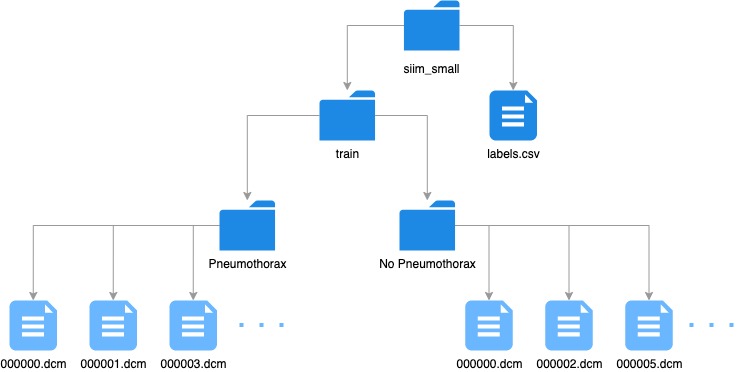
The *siim_small* folder has the following directory/file structure:

<figure>
<img src="images/siim_folder_structure.jpeg"
alt="siim_folder_structure.jpg" />
<figcaption aria-hidden="true">siim_folder_structure.jpg</figcaption>
</figure>

## What are DICOMs?

**DICOM**(**D**igital **I**maging and **CO**mmunications in
**M**edicine) is the de-facto standard that establishes rules that allow
medical images(X-Ray, MRI, CT) and associated information to be
exchanged between imaging equipment from different vendors, computers,
and hospitals. The DICOM format provides a suitable means that meets
health infomation exchange (HIE) standards for transmision of health
related data among facilites and HL7 standards which is the messaging
standard that enables clinical applications to exchange data

DICOM files typically have a `.dcm` extension and provides a means of
storing data in separate ‘tags’ such as patient information as well as
image/pixel data. A DICOM file consists of a header and image data sets
packed into a single file. By extracting data from these tags one can
access important information regarding the patient demographics, study
parameters, etc.

16 bit DICOM images have values ranging from `-32768` to `32768` while
8-bit greyscale images store values from `0` to `255`. The value ranges
in DICOM images are useful as they correlate with the [Hounsfield
Scale](https://en.wikipedia.org/wiki/Hounsfield_scale) which is a
quantitative scale for describing radiodensity

### Plotting the DICOM data

To analyze our dataset, we load the paths to the DICOM files with the
[`get_dicom_files`](https://docs.fast.ai/medical.imaging.html#get_dicom_files)
function. When calling the function, we append *train/* to the
`pneumothorax_source` path to choose the folder where the DICOM files
are located. We store the path to each DICOM file in the `items` list.

``` python
items = get_dicom_files(pneumothorax_source/f"train/")
```

Next, we split the `items` list into a train `trn` and validation `val`
list using the
[`RandomSplitter`](https://docs.fast.ai/data.transforms.html#randomsplitter)
function:

``` python
trn,val = RandomSplitter()(items)
```

Pydicom is a python package for parsing DICOM files, making it easier to
access the `header` of the DICOM as well as coverting the raw
`pixel_data` into pythonic structures for easier manipulation.
`fastai.medical.imaging` uses `pydicom.dcmread` to load the DICOM file.

To plot an X-ray, we can select an entry in the `items` list and load
the DICOM file with `dcmread`.

``` python
patient = 7
xray_sample = items[patient].dcmread()
```

To view the `header`

``` python
xray_sample
```

    Dataset.file_meta -------------------------------
    (0002, 0000) File Meta Information Group Length  UL: 200
    (0002, 0001) File Meta Information Version       OB: b'\x00\x01'
    (0002, 0002) Media Storage SOP Class UID         UI: Secondary Capture Image Storage
    (0002, 0003) Media Storage SOP Instance UID      UI: 1.2.276.0.7230010.3.1.4.8323329.3297.1517875177.149805
    (0002, 0010) Transfer Syntax UID                 UI: JPEG Baseline (Process 1)
    (0002, 0012) Implementation Class UID            UI: 1.2.276.0.7230010.3.0.3.6.0
    (0002, 0013) Implementation Version Name         SH: 'OFFIS_DCMTK_360'
    -------------------------------------------------
    (0008, 0005) Specific Character Set              CS: 'ISO_IR 100'
    (0008, 0016) SOP Class UID                       UI: Secondary Capture Image Storage
    (0008, 0018) SOP Instance UID                    UI: 1.2.276.0.7230010.3.1.4.8323329.3297.1517875177.149805
    (0008, 0020) Study Date                          DA: '19010101'
    (0008, 0030) Study Time                          TM: '000000.00'
    (0008, 0050) Accession Number                    SH: ''
    (0008, 0060) Modality                            CS: 'CR'
    (0008, 0064) Conversion Type                     CS: 'WSD'
    (0008, 0090) Referring Physician's Name          PN: ''
    (0008, 103e) Series Description                  LO: 'view: PA'
    (0010, 0010) Patient's Name                      PN: '6633c659-9249-443e-9851-b83782d1b111'
    (0010, 0020) Patient ID                          LO: '6633c659-9249-443e-9851-b83782d1b111'
    (0010, 0030) Patient's Birth Date                DA: ''
    (0010, 0040) Patient's Sex                       CS: 'M'
    (0010, 1010) Patient's Age                       AS: '21'
    (0018, 0015) Body Part Examined                  CS: 'CHEST'
    (0018, 5101) View Position                       CS: 'PA'
    (0020, 000d) Study Instance UID                  UI: 1.2.276.0.7230010.3.1.2.8323329.3297.1517875177.149804
    (0020, 000e) Series Instance UID                 UI: 1.2.276.0.7230010.3.1.3.8323329.3297.1517875177.149803
    (0020, 0010) Study ID                            SH: ''
    (0020, 0011) Series Number                       IS: "1"
    (0020, 0013) Instance Number                     IS: "1"
    (0020, 0020) Patient Orientation                 CS: ''
    (0028, 0002) Samples per Pixel                   US: 1
    (0028, 0004) Photometric Interpretation          CS: 'MONOCHROME2'
    (0028, 0010) Rows                                US: 1024
    (0028, 0011) Columns                             US: 1024
    (0028, 0030) Pixel Spacing                       DS: [0.14300000000000002, 0.14300000000000002]
    (0028, 0100) Bits Allocated                      US: 8
    (0028, 0101) Bits Stored                         US: 8
    (0028, 0102) High Bit                            US: 7
    (0028, 0103) Pixel Representation                US: 0
    (0028, 2110) Lossy Image Compression             CS: '01'
    (0028, 2114) Lossy Image Compression Method      CS: 'ISO_10918_1'
    (7fe0, 0010) Pixel Data                          OB: Array of 161452 elements

Explanation of each element is beyond the scope of this tutorial but
[this](http://dicom.nema.org/medical/dicom/current/output/chtml/part03/sect_C.7.6.3.html#sect_C.7.6.3.1.4)
site has some excellent information about each of the entries

Some key pointers on the tag information above:

- **Pixel Data** (7fe0 0010) - This is where the raw pixel data is
  stored. The order of pixels encoded for each image plane is left to
  right, top to bottom, i.e., the upper left pixel (labeled 1,1) is
  encoded first
- **Photometric Interpretation** (0028, 0004) - also known as color
  space. In this case it is `MONOCHROME2` where pixel data is
  represented as a single monochrome image plane where low values=dark,
  high values=bright. If the colorspace was `MONOCHROME` then the low
  values=bright and high values=dark info.
- **Samples per Pixel** (0028, 0002) - This should be 1 as this image is
  monochrome. This value would be 3 if the color space was RGB for
  example
- **Bits Stored** (0028 0101) - Number of bits stored for each pixel
  sample. Typical 8 bit images have a pixel range between `0` and `255`
- **Pixel Represenation**(0028 0103) - can either be unsigned(0) or
  signed(1)
- **Lossy Image Compression** (0028 2110) - `00` image has not been
  subjected to lossy compression. `01` image has been subjected to lossy
  compression.
- **Lossy Image Compression Method** (0028 2114) - states the type of
  lossy compression used (in this case `ISO_10918_1` represents JPEG
  Lossy Compression)
- **Pixel Data** (7fe0, 0010) - Array of 161452 elements represents the
  image pixel data that pydicom uses to convert the pixel data into an
  image.

What does `PixelData` look like?

``` python
xray_sample.PixelData[:200]
```

    b'\xfe\xff\x00\xe0\x00\x00\x00\x00\xfe\xff\x00\xe0\x9cv\x02\x00\xff\xd8\xff\xdb\x00C\x00\x03\x02\x02\x02\x02\x02\x03\x02\x02\x02\x03\x03\x03\x03\x04\x06\x04\x04\x04\x04\x04\x08\x06\x06\x05\x06\t\x08\n\n\t\x08\t\t\n\x0c\x0f\x0c\n\x0b\x0e\x0b\t\t\n\x11\n\x0e\x0f\x10\x10\x11\x10\n\x0c\x12\x13\x12\x10\x13\x0f\x10\x10\x10\xff\xc0\x00\x0b\x08\x04\x00\x04\x00\x01\x01\x11\x00\xff\xc4\x00\x1d\x00\x00\x02\x03\x01\x01\x01\x01\x01\x00\x00\x00\x00\x00\x00\x00\x00\x04\x05\x02\x03\x06\x00\x01\x07\x08\t\xff\xc4\x00R\x10\x00\x02\x01\x03\x03\x02\x04\x03\x06\x05\x04\x00\x04\x01\x02\x17\x01\x02\x11\x00\x03!\x04\x121\x05A\x13"Qa\x06q\x81\x142\x91\xa1\xb1\xf0#B\xc1\xd1\xe1\x07\x15R\xf1\x16$3br\x08%4C&cs\x82\x92\xa2'

Because of the complexity in interpreting `PixelData`, pydicom provides
an easy way to get it in a convenient form: `pixel_array` which returns
a `numpy.ndarray` containing the pixel data:

``` python
xray_sample.pixel_array, xray_sample.pixel_array.shape
```

    (array([[ 0,  0,  0, ..., 13, 13,  5],
            [ 0,  0,  0, ..., 13, 13,  5],
            [ 0,  0,  0, ..., 13, 12,  5],
            ...,
            [ 0,  0,  0, ...,  5,  3,  0],
            [ 0,  0,  0, ...,  6,  4,  0],
            [ 0,  0,  0, ...,  8,  5,  0]], dtype=uint8),
     (1024, 1024))

You can then use the `show` function to view the image

``` python
xray_sample.show()
```

![](61_tutorial.medical_imaging_files/figure-commonmark/cell-11-output-1.svg)

You can also conveniently create a dataframe with all the `tag`
information as columns for all the images in a dataset by using
`from_dicoms`

``` python
dicom_dataframe = pd.DataFrame.from_dicoms(items)
dicom_dataframe[:5]
```

<div>
<style scoped>
    .dataframe tbody tr th:only-of-type {
        vertical-align: middle;
    }
&#10;    .dataframe tbody tr th {
        vertical-align: top;
    }
&#10;    .dataframe thead th {
        text-align: right;
    }
</style>

<table class="dataframe" data-quarto-postprocess="true" data-border="1">
<thead>
<tr style="text-align: right;">
<th data-quarto-table-cell-role="th"></th>
<th data-quarto-table-cell-role="th">SpecificCharacterSet</th>
<th data-quarto-table-cell-role="th">SOPClassUID</th>
<th data-quarto-table-cell-role="th">SOPInstanceUID</th>
<th data-quarto-table-cell-role="th">StudyDate</th>
<th data-quarto-table-cell-role="th">StudyTime</th>
<th data-quarto-table-cell-role="th">AccessionNumber</th>
<th data-quarto-table-cell-role="th">Modality</th>
<th data-quarto-table-cell-role="th">ConversionType</th>
<th data-quarto-table-cell-role="th">ReferringPhysicianName</th>
<th data-quarto-table-cell-role="th">SeriesDescription</th>
<th data-quarto-table-cell-role="th">...</th>
<th data-quarto-table-cell-role="th">LossyImageCompression</th>
<th data-quarto-table-cell-role="th">LossyImageCompressionMethod</th>
<th data-quarto-table-cell-role="th">fname</th>
<th data-quarto-table-cell-role="th">MultiPixelSpacing</th>
<th data-quarto-table-cell-role="th">PixelSpacing1</th>
<th data-quarto-table-cell-role="th">img_min</th>
<th data-quarto-table-cell-role="th">img_max</th>
<th data-quarto-table-cell-role="th">img_mean</th>
<th data-quarto-table-cell-role="th">img_std</th>
<th data-quarto-table-cell-role="th">img_pct_window</th>
</tr>
</thead>
<tbody>
<tr>
<td data-quarto-table-cell-role="th">0</td>
<td>ISO_IR 100</td>
<td>1.2.840.10008.5.1.4.1.1.7</td>
<td>1.2.276.0.7230010.3.1.4.8323329.6904.1517875201.850819</td>
<td>19010101</td>
<td>000000.00</td>
<td></td>
<td>CR</td>
<td>WSD</td>
<td></td>
<td>view: PA</td>
<td>...</td>
<td>01</td>
<td>ISO_10918_1</td>
<td>C:\Users\tijme\.fastai\data\siim_small\train\No
Pneumothorax\000000.dcm</td>
<td>1</td>
<td>0.168</td>
<td>0</td>
<td>254</td>
<td>160.398039</td>
<td>53.854885</td>
<td>0.087029</td>
</tr>
<tr>
<td data-quarto-table-cell-role="th">1</td>
<td>ISO_IR 100</td>
<td>1.2.840.10008.5.1.4.1.1.7</td>
<td>1.2.276.0.7230010.3.1.4.8323329.11028.1517875229.983789</td>
<td>19010101</td>
<td>000000.00</td>
<td></td>
<td>CR</td>
<td>WSD</td>
<td></td>
<td>view: PA</td>
<td>...</td>
<td>01</td>
<td>ISO_10918_1</td>
<td>C:\Users\tijme\.fastai\data\siim_small\train\No
Pneumothorax\000002.dcm</td>
<td>1</td>
<td>0.143</td>
<td>0</td>
<td>250</td>
<td>114.524713</td>
<td>70.752315</td>
<td>0.326269</td>
</tr>
<tr>
<td data-quarto-table-cell-role="th">2</td>
<td>ISO_IR 100</td>
<td>1.2.840.10008.5.1.4.1.1.7</td>
<td>1.2.276.0.7230010.3.1.4.8323329.11444.1517875232.977506</td>
<td>19010101</td>
<td>000000.00</td>
<td></td>
<td>CR</td>
<td>WSD</td>
<td></td>
<td>view: PA</td>
<td>...</td>
<td>01</td>
<td>ISO_10918_1</td>
<td>C:\Users\tijme\.fastai\data\siim_small\train\No
Pneumothorax\000005.dcm</td>
<td>1</td>
<td>0.143</td>
<td>0</td>
<td>246</td>
<td>132.218334</td>
<td>73.023531</td>
<td>0.266901</td>
</tr>
<tr>
<td data-quarto-table-cell-role="th">3</td>
<td>ISO_IR 100</td>
<td>1.2.840.10008.5.1.4.1.1.7</td>
<td>1.2.276.0.7230010.3.1.4.8323329.32219.1517875159.70802</td>
<td>19010101</td>
<td>000000.00</td>
<td></td>
<td>CR</td>
<td>WSD</td>
<td></td>
<td>view: PA</td>
<td>...</td>
<td>01</td>
<td>ISO_10918_1</td>
<td>C:\Users\tijme\.fastai\data\siim_small\train\No
Pneumothorax\000006.dcm</td>
<td>1</td>
<td>0.171</td>
<td>0</td>
<td>255</td>
<td>153.405355</td>
<td>59.543063</td>
<td>0.144505</td>
</tr>
<tr>
<td data-quarto-table-cell-role="th">4</td>
<td>ISO_IR 100</td>
<td>1.2.840.10008.5.1.4.1.1.7</td>
<td>1.2.276.0.7230010.3.1.4.8323329.32395.1517875160.396775</td>
<td>19010101</td>
<td>000000.00</td>
<td></td>
<td>CR</td>
<td>WSD</td>
<td></td>
<td>view: PA</td>
<td>...</td>
<td>01</td>
<td>ISO_10918_1</td>
<td>C:\Users\tijme\.fastai\data\siim_small\train\No
Pneumothorax\000007.dcm</td>
<td>1</td>
<td>0.171</td>
<td>0</td>
<td>250</td>
<td>166.198407</td>
<td>50.008985</td>
<td>0.053009</td>
</tr>
</tbody>
</table>

<p>5 rows × 42 columns</p>
</div>

Next, we need to load the labels for the dataset. We import the
*labels.csv* file using pandas and print the first five entries. The
**file** column shows the relative path to the *.dcm* file and the
**label** column indicates whether the chest x-ray has a pneumothorax or
not.

``` python
df = pd.read_csv(pneumothorax_source/f"labels.csv")
df.head()
```

<div>
<style scoped>
    .dataframe tbody tr th:only-of-type {
        vertical-align: middle;
    }
&#10;    .dataframe tbody tr th {
        vertical-align: top;
    }
&#10;    .dataframe thead th {
        text-align: right;
    }
</style>

<table class="dataframe" data-quarto-postprocess="true" data-border="1">
<thead>
<tr style="text-align: right;">
<th data-quarto-table-cell-role="th"></th>
<th data-quarto-table-cell-role="th">file</th>
<th data-quarto-table-cell-role="th">label</th>
</tr>
</thead>
<tbody>
<tr>
<td data-quarto-table-cell-role="th">0</td>
<td>train/No Pneumothorax/000000.dcm</td>
<td>No Pneumothorax</td>
</tr>
<tr>
<td data-quarto-table-cell-role="th">1</td>
<td>train/Pneumothorax/000001.dcm</td>
<td>Pneumothorax</td>
</tr>
<tr>
<td data-quarto-table-cell-role="th">2</td>
<td>train/No Pneumothorax/000002.dcm</td>
<td>No Pneumothorax</td>
</tr>
<tr>
<td data-quarto-table-cell-role="th">3</td>
<td>train/Pneumothorax/000003.dcm</td>
<td>Pneumothorax</td>
</tr>
<tr>
<td data-quarto-table-cell-role="th">4</td>
<td>train/Pneumothorax/000004.dcm</td>
<td>Pneumothorax</td>
</tr>
</tbody>
</table>

</div>

Now, we use the
[`DataBlock`](https://docs.fast.ai/data.block.html#datablock) class to
prepare the DICOM data for training.

As we are dealing with DICOM images, we need to use
[`PILDicom`](https://docs.fast.ai/medical.imaging.html#pildicom) as the
[`ImageBlock`](https://docs.fast.ai/vision.data.html#imageblock)
category. This is so the
[`DataBlock`](https://docs.fast.ai/data.block.html#datablock) will know
how to open the DICOM images. As this is a binary classification task we
will use
[`CategoryBlock`](https://docs.fast.ai/data.block.html#categoryblock)

``` python
pneumothorax = DataBlock(blocks=(ImageBlock(cls=PILDicom), CategoryBlock),
                   get_x=lambda x:pneumothorax_source/f"{x[0]}",
                   get_y=lambda x:x[1],
                   batch_tfms=[*aug_transforms(size=224),Normalize.from_stats(*imagenet_stats)])

dls = pneumothorax.dataloaders(df.values, num_workers=0)
```

Additionally, we plot a first batch with the specified transformations:

``` python
dls = pneumothorax.dataloaders(df.values)
dls.show_batch(max_n=16)
```

    Due to IPython and Windows limitation, python multiprocessing isn't available now.
    So `number_workers` is changed to 0 to avoid getting stuck

![](61_tutorial.medical_imaging_files/figure-commonmark/cell-15-output-2.svg)

## Training

We can then use the
[`vision_learner`](https://docs.fast.ai/vision.learner.html#vision_learner)
function and initiate the training.

``` python
learn = vision_learner(dls, resnet34, metrics=accuracy)
```

Note that if you do not select a loss or optimizer function, fastai will
try to choose the best selection for the task. You can check the loss
function by calling `loss_func`

``` python
learn.loss_func
```

    FlattenedLoss of CrossEntropyLoss()

And you can do the same for the optimizer by calling `opt_func`

``` python
learn.opt_func
```

    <function fastai.optimizer.Adam(params, lr, mom=0.9, sqr_mom=0.99, eps=1e-05, wd=0.01, decouple_wd=True)>

Use `lr_find` to try to find the best learning rate

``` python
learn.lr_find()
```

    <div>
        <style>
            /* Turns off some styling */
            progress {
                /* gets rid of default border in Firefox and Opera. */
                border: none;
                /* Needs to be in here for Safari polyfill so background images work as expected. */
                background-size: auto;
            }
            .progress-bar-interrupted, .progress-bar-interrupted::-webkit-progress-bar {
                background: #F44336;
            }
        </style>
      <progress value='0' class='' max='34' style='width:300px; height:20px; vertical-align: middle;'></progress>
      &#10;    </div>
    &#10;

    SuggestedLRs(lr_min=0.005754399299621582, lr_steep=0.0063095735386013985)

![](61_tutorial.medical_imaging_files/figure-commonmark/cell-19-output-3.svg)

``` python
learn.fit_one_cycle(1)
```

<table class="dataframe" data-quarto-postprocess="true" data-border="1">
<thead>
<tr style="text-align: left;">
<th data-quarto-table-cell-role="th">epoch</th>
<th data-quarto-table-cell-role="th">train_loss</th>
<th data-quarto-table-cell-role="th">valid_loss</th>
<th data-quarto-table-cell-role="th">accuracy</th>
<th data-quarto-table-cell-role="th">time</th>
</tr>
</thead>
<tbody>
<tr>
<td>0</td>
<td>1.191782</td>
<td>2.123666</td>
<td>0.320000</td>
<td>00:37</td>
</tr>
</tbody>
</table>

``` python
learn.predict(pneumothorax_source/f"train/Pneumothorax/000004.dcm")
```

When predicting on an image `learn.predict` returns a tuple (class,
class tensor and \[probabilities of each class\]).In this dataset there
are only 2 classes `No Pneumothorax` and `Pneumothorax` hence the reason
why each probability has 2 values, the first value is the probability
whether the image belongs to `class 0` or `No Pneumothorax` and the
second value is the probability whether the image belongs to `class 1`
or `Pneumothorax`

``` python
tta = learn.tta(use_max=True)
```

    <div>
        <style>
            /* Turns off some styling */
            progress {
                /* gets rid of default border in Firefox and Opera. */
                border: none;
                /* Needs to be in here for Safari polyfill so background images work as expected. */
                background-size: auto;
            }
            .progress-bar-interrupted, .progress-bar-interrupted::-webkit-progress-bar {
                background: #F44336;
            }
        </style>
      <progress value='0' class='' max='1' style='width:300px; height:20px; vertical-align: middle;'></progress>
      &#10;    </div>
    

``` python
learn.show_results(max_n=16)
```

    <div>
        <style>
            /* Turns off some styling */
            progress {
                /* gets rid of default border in Firefox and Opera. */
                border: none;
                /* Needs to be in here for Safari polyfill so background images work as expected. */
                background-size: auto;
            }
            .progress-bar-interrupted, .progress-bar-interrupted::-webkit-progress-bar {
                background: #F44336;
            }
        </style>
      <progress value='0' class='' max='1' style='width:300px; height:20px; vertical-align: middle;'></progress>
      &#10;    </div>
    &#10;

![](61_tutorial.medical_imaging_files/figure-commonmark/cell-23-output-2.svg)

``` python
interp = Interpretation.from_learner(learn)
```

``` python
interp.plot_top_losses(2)
```

![](61_tutorial.medical_imaging_files/figure-commonmark/cell-25-output-1.svg)

## Result Evaluation

Medical models are predominantly high impact so it is important to know
how good a model is at detecting a certain condition.

This model has an accuracy of 56%. Accuracy can be defined as the number
of correctly predicted data points out of all the data points. However
in this context we can define accuracy as the probability that the model
is correct and the patient has the condition **PLUS** the probability
that the model is correct and the patient does not have the condition

There are some other key terms that need to be used when evaluating
medical models:

**False Positive & False Negative**

- **False Positive** is an error in which a test result improperly
  indicates presence of a condition, such as a disease (the result is
  positive), when in reality it is not present

- **False Negative** is an error in which a test result improperly
  indicates no presence of a condition (the result is negative), when in
  reality it is present

**Sensitivity & Specificity**

- **Sensitivity or True Positive Rate** is where the model classifies a
  patient has the disease given the patient actually does have the
  disease. Sensitivity quantifies the avoidance of false negatives

Example: A new test was tested on 10,000 patients, if the new test has a
sensitivity of 90% the test will correctly detect 9,000 (True Positive)
patients but will miss 1000 (False Negative) patients that have the
condition but were tested as not having the condition

- **Specificity or True Negative Rate** is where the model classifies a
  patient as not having the disease given the patient actually does not
  have the disease. Specificity quantifies the avoidance of false
  positives

[Understanding and using sensitivity, specificity and predictive
values](https://www.ncbi.nlm.nih.gov/pmc/articles/PMC2636062/) is a
great paper if you are interested in learning more about understanding
sensitivity, specificity and predictive values.

**PPV and NPV**

Most medical testing is evaluated via **PPV** (Positive Predictive
Value) or **NPV** (Negative Predictive Value).

**PPV** - if the model predicts a patient has a condition what is the
probability that the patient actually has the condition

**NPV** - if the model predicts a patient does not have a condition what
is the probability that the patient actually does not have the condition

The ideal value of the PPV, with a perfect test, is 1 (100%), and the
worst possible value would be zero

The ideal value of the NPV, with a perfect test, is 1 (100%), and the
worst possible value would be zero

**Confusion Matrix**

The confusion matrix is plotted against the `valid` dataset

``` python
interp = ClassificationInterpretation.from_learner(learn)
losses,idxs = interp.top_losses()
len(dls.valid_ds)==len(losses)==len(idxs)
interp.plot_confusion_matrix(figsize=(7,7))
```

![](61_tutorial.medical_imaging_files/figure-commonmark/cell-26-output-2.png)

You can also reproduce the results interpreted from
plot_confusion_matrix like so:

``` python
upp, low = interp.confusion_matrix()
tn, fp = upp[0], upp[1]
fn, tp = low[0], low[1]
print(tn, fp, fn, tp)
```

    23 13 12 2

Note that **Sensitivity = True Positive/(True Positive + False
Negative)**

``` python
sensitivity = tp/(tp + fn)
sensitivity
```

    0.14285714285714285

In this case the model has a sensitivity of 40% and hence is only
capable of correctly detecting 40% True Positives (i.e. who have
Pneumothorax) but will miss 60% of False Negatives (patients that
actually have Pneumothorax but were told they did not! Not a good
situation to be in).

This is also know as a **Type II error**

**Specificity = True Negative/(False Positive + True Negative)**

``` python
specificity = tn/(fp + tn)
specificity
```

    0.6388888888888888

The model has a specificity of 63% and hence can correctly detect 63% of
the time that a patient does **not** have Pneumothorax but will
incorrectly classify that 37% of the patients have Pneumothorax (False
Postive) but actually do not.

This is also known as a **Type I error**

**Positive Predictive Value (PPV)**

``` python
ppv = tp/(tp+fp)
ppv
```

    0.13333333333333333

In this case the model performs poorly in correctly predicting patients
with Pneumothorax

**Negative Predictive Value (NPV)**

``` python
npv = tn/(tn+fn)
npv
```

    0.6571428571428571

This model is better at predicting patients with No Pneumothorax

**Calculating Accuracy**

The accuracy of this model as mentioned before was 56% but how was this
calculated? We can consider accuracy as:

**accuracy = sensitivity x prevalence + specificity \* (1 -
prevalence)**

Where **prevalence** is a statistical concept referring to the number of
cases of a disease that are present in a particular population at a
given time. The prevalence in this case is how many patients in the
valid dataset have the condition compared to the total number.

To view the files in the valid dataset you call `dls.valid_ds.cat`

``` python
val = dls.valid_ds.cat
#val[0]
```

There are 15 Pneumothorax images in the valid set (which has a total of
50 images and can be checked by using `len(dls.valid_ds)`) so the
prevalence here is 15/50 = 0.3

``` python
prevalence = 15/50
prevalence
```

    0.3

``` python
accuracy = (sensitivity * prevalence) + (specificity * (1 - prevalence))
accuracy
```

    0.490079365079365

***Citations:***

\[1\] *Filice R et al. Crowdsourcing pneumothorax annotations using
machine learning annotations on the NIH chest X-ray dataset. J Digit
Imaging (2019). https://doi.org/10.1007/s10278-019-00299-9*